T-tests allow us to take two groups of samples and check if there is a significant enough difference between them. As a hypothesis testing tool, they can be used to determine whether the observed irregularity is a coincidence, or if it can be transposed to the entire population.

To exemplify, let’s say we have a crop field to which we are going to apply a new type of fertilizer. In order to tell if the chemical has an effect on the harvest, we will take a sample of crops before the treatment, and then another one after. Running a t-test on the samples will tell us if there is a substantial difference between “before” and “after”, and if the findings are valid for the whole field.

This post examines how t-tests are performed using t-values and t-distributions, which will help us understand probability calculation and hypothesis assessment.

We’ll focus on clear explanations of the core concepts — t-values and t-distributions — and use graphs rather than numbers and equations for illustration.

What Are t-Values?

The very term t-test reflects that the test results are based purely on t-values. T-value is what statisticians refer to as a test statistic, and it is calculated from your sample data during hypothesis tests. It is then used to compare your data to what is expected under s.c. null hypothesis. If the resulting t-value is extreme enough, it means that you have encountered a deviation from the null hypothesis, significant enough to allow you to reject the null.

The way it works is as follows. During any type of t-test, your sample data (size and variability) is processed and distilled to a single number – the t-value. The result equal to zero means that your data matches the null hypothesis and there are no irregularities found. The increase in the absolute value of the t-value signifies that the difference between the sample data and the null hypothesis is also increasing.

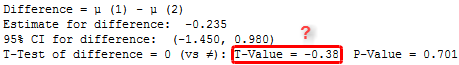
However, the analysis doesn’t stop there. The difficulty is that the t-value is a unitless statistic and isn’t very informative by itself. Say, for instance, the calculations performed under a t-test resulted in a t-value of 2. In this case, we know that there is a difference from the null hypothesis because the result is not zero. But just how common or rare is this difference, given that the null hypothesis is correct? “2” tells us nothing about that.

In order to make any assumptions in this regard, we need to look at the t-value in a broader context. Such as provided by t-distributions.

What Are t-Distributions?

The first concept we need to familiarize ourselves with is a sampling distribution. Here is the basic idea. A single t-test generates a single t-value. So, to get distribution, we need to take multiple random samples of equal size from the same population and feed them through the same t-test. This way we will get a spread of t-values, which can be plotted as a sampling distribution – a special case of probability distributions.

Afterward, the plotting process is rather straight-forward. The properties of t-distributions are well-understood and you don’t need to collect too many samples to complete the task. What defines any specific t-distribution is its degrees of freedom (DF). This value is closely related to sample size, therefore, t-distribution characteristics will differ depending on the sample size we choose to work with.

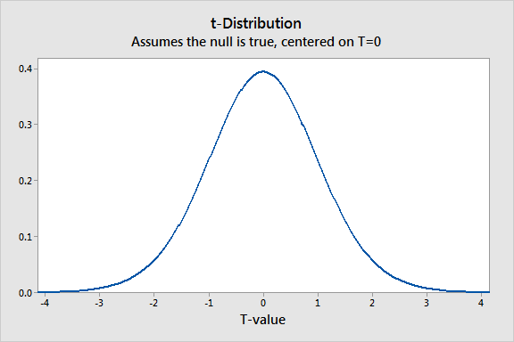
A visual representation of t-distribution is a graph showing a spread of t-values obtained from a population where the null hypothesis is true. The sampling distribution is used to estimate the consistency of your results against the null theory.

Using t-Distribution to Check Your Sample Results Against the Null Hypothesis

When we process a random set of samples from a certain population and plot a t-distribution, we assume that the null hypothesis is correct for this population. To find out how much your data deviates from the null hypothesis, apply your study’s t-value to the t-distribution.

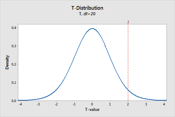
The sampling distribution graph above shows a t-distribution with 20 degrees of freedom. This corresponds to a sample size of 21 in a one-sample t-test. The fact that the graph peaks right at zero indicate that we are most likely to obtain a t-value close to the null hypothesis, and least likely the further we move away from zero in either direction. This is evident from the assumption that the null hypothesis is true.

The hypothetical value of 2 that we assumed earlier is marked on the graph, and it demonstrates where our sample data is located compared to the null hypothesis. We see that, even though the probability isn’t very high, there is a fair chance of detecting a t-value from -2 to +2.

So, there is a positive difference between our sample data and the null-hypothesis. OK. And we see that the t-value of 2 is rare. So far so good. But we still don’t know how rare it is precisely. Ultimately, in the scope of this analysis, we want to be able to tell if our findings are exceptional enough to justify rejecting the null hypothesis. We’ll be able to do this after we’ve calculated the probability.

How to Use t-Values and t-Distributions to Calculate Probabilities

Performing any hypothesis test implies taking the test statistic from a specific sample and placing it within the context of a known probability distribution. T-tests are no exception: taking a t-value and placing it in the context of the calculated t-distribution enables you to derive the probabilities associated with that t-value. In case a t-value is exceptional enough when the null hypothesis is true, we can reject the null.

Before we proceed with calculating the probability associated with our hypothetical value of 2, there are two critical points to clarify.

1. We’ll be using t-values of +2 and -2 because we are currently looking at the results of s.c. two-tailed test. This type of tests lets you evaluate if the sample average is greater or less than the target value in a 1-sample t-test. A one-tail t-test will only show a difference either in a positive or negative direction.
2. It is only possible to calculate a meaningful probability for a range of t-values. As we see in the graph below, a range of t-values corresponds to a specific area shaded under a distribution curve – that’s the probability. The probability for a single point equals zero because a single point creates no such area.

Interpreting t-Test Results for Our Hypothetical Example

With these points in mind, we’re able to read the graph below: it shows the probability associated with t-values less than -2 and greater than +2. The graph corresponds to our t-test design (1-sample t-test, with the number of samples of 21).

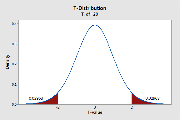
To interpret this distribution plot we say that each shaded region has a probability of 0.02963, meaning the total probability is 0.05926. We can also conclude that t-values will fall within these areas near 6% of the time, given the null hypothesis is true.

Some of you may already be familiar with this type of probability – it’s called the p-value. It’s fair to say that the chances of t-values falling within these regions seem low. However, it’s not quite low enough to reject the null hypothesis, applying the general significance level of 0.05.

t-Distributions and Sample Size

As previously mentioned, t-distributions are determined by the degrees of freedom, which are closely related to sample size. The more the DF increases, the more the probability density in the tails decreases. Along with that the distribution becomes more tightly grouped around the central mark.

Bulkier tails mean that there is a greater chance of t-values being far removed from zero, even when the null hypothesis is true. Such shape variation is a means for t-distributions to respond to growing uncertainty that stems from processing smaller samples.

The graph below displays the difference in probability distribution plots between t-distributions for 5 and 30 DF.

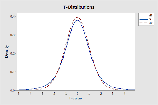
Averages from smaller samples are usually less accurate. The reason is it’s less unlikely to get an exceptional t-value with a smaller sample. This has a direct effect on both p-values and probabilities. To exemplify, a t-value of 2 in a two-tailed test for 5 and 30 DF will have p-values of 10.2% and 5.4% accordingly. The bottom line is whenever possible, aim at using bigger samples.

Conclusion

Whether you have to compare a sample mean to a hypothesized or target value, compare means of two independent samples, or find a difference between paired samples, there are specific types of t-tests that will allow you to do just that. Conveniently, there are also tools (such as QuickCalcs by GraphPad) you can use to perform the necessary calculations.

With this guide, we wanted to provide a clear, down-to-earth explanation of what t-tests are, as well as to show the basics of how to run them and interpret the results. Let us know if you found it helpful, and please, feel free to explore our blog further for more great content! In case you need help on any data research or analytics project, get in touch with us for full assistance!

Related articles:

What Are the “HTTP” and “WWW” in URLs? Are they required?

Share on: